# 【工具曲线参考】
# Intro
When writing shader or during any procedural creation process (texturing, modeling, shading, animation...) you often find yourself modifying signals in different ways so they behave the way you need. It is common to use smoothstep() to threshold some values, or pow() to shape a signal, or clamp() to clip it, fmod() to make it repeat, a mix() to blend between two signals, exp() for attenuatation, etc etc. All these functions are often conveniently available by default in most languages. However there are some operations that are also relativelly used that don't come by default in any language. The following is a list of some of the functions that I find myself using over and over again:
# Almost Identity (I)
Imagine you don't want to modify a signal unless it's drops to zero or close to it, in which case you want to replace the value with a small possitive constant. Then, rather than clamping the value and introduce a discontinuity, you can smoothly blend the signal into the desired clipped value. So, let m be the threshold (anything above m stays unchanged), and n the value things will take when the signal is zero. Then, the following function does the soft clipping (in a cubic fashion):
float almostIdentity( float x, float m, float n )
{
    if( x>m ) return x;
    const float a = 2.0*n - m;
    const float b = 2.0*m - 3.0*n;
    const float t = x/m;
    return (a*t + b)*t*t + n;
}
# Almost Identity (II)
A different way to achieve a near identity is through the square root of a biased square. I saw this technique first in a shader by user "omeometo" in Shadertoy. This approach can be a bit slower than the cubic above, depending on the hardware, but I find myself using it a lot these days. While it has zero derivative, it has a non-zero second derivative, so keep an eye in case it causes problems in your application.
An extra nice thing is that this function can be used, unaltered, as an smooth-abs() function, which comes handy for symmetric funtions such as mirrored SDFs.
float almostIdentity( float x, float n )
{
    return sqrt(x*x+n);
}
# Almost Unit Identity
This is a near-identiy function that maps the unit interval into itself. It is the cousin of smoothstep(), in that it maps 0 to 0, 1 to 1, and has a 0 derivative at the origin, just like smoothstep. However, instead of having a 0 derivative at 1, it has a derivative of 1 at that point.It's equivalent to the Almost Identiy above with n=0 and m=1. Since it's a cubic just like smoothstep() it is very fast to evaluate:
float almostUnitIdentity( float x )
{
    return x*x*(2.0-x);
}
# Smoothstep Integral
If you use smoothstep for a velocity signal (say, you want to smoothly accelerate a stationary object into constant velocity motion), you need to integrate smoothstep() over time in order to get the actual position of value of the animation. The function below is exactly that, the position of an object that accelerates with smoothstep. Note it's derivative is never larger than 1, so no decelerations happen.
float integralSmoothstep( float x, float T )
{
    if( x>T ) return x - T/2.0;
    return x*x*x*(1.0-x*0.5/T)/T/T;
}
# Exponential Impulse
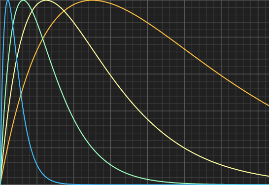
Impulses are great for triggering behaviours or making envelopes for music or animation. Baiscally, for anything that grows fast and then decays slowly. The following is an exponential impulse function. Use k to control the stretching of the function. Its maximum, which is 1, happens at exactly x = 1/k.
float expImpulse( float x, float k )
{
    const float h = k*x;
    return h*exp(1.0-h);
}
# Polynomial Impulse
Another impulse function that doesn't use exponentials can be designed by using polynomials. Use k to control falloff of the function. For example, a quadratic can be used, which peaks at x = sqrt(1/k).
float quaImpulse( float k, float x )
{
    return 2.0*sqrt(k)*x/(1.0+k*x*x);
}
You can easily generalize it to other powers to get different falloff shapes, where n is the degree of the polynomial:
float polyImpulse( float k, float n, float x )
{
    return (n/(n-1.0))*pow((n-1.0)*k,1.0/n)*x/(1.0+k*pow(x,n));
}
These generalized impulses peak at x = [k(n-1)] ^-1/n^ .
# Sustained Impulse
Similar to the previous, but it allows for control on the width of attack (through the parameter "k") and the release (parameter "f") independently. Also, the impulse releases at a value of 1 instead of 0.
float expSustainedImpulse( float x, float f, float k )
{
    float s = max(x-f,0.0)
    return min( x*x/(f*f), 1+(2.0/f)*s*exp(-k*s));
}
# Cubic Pulse
Chances are you found yourself doing smoothstep(c-w,c,x)-smoothstep(c,c+w,x) very often. I do, for example when I need to isolate some features in a signal. For those cases, this cubicPulse() below is my new friend and will be yours too soon. Bonus - you can also use it as a performant replacement for a gaussian.
float cubicPulse( float c, float w, float x )
{
    x = fabs(x - c);
    if( x>w ) return 0.0;
    x /= w;
    return 1.0 - x*x*(3.0-2.0*x);
}
# Exponential Step
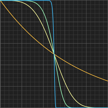
A natural attenuation is an exponential of a linearly decaying quantity: yellow curve, exp(-x). A gaussian, is an exponential of a quadratically decaying quantity: light green curve, exp(-x ^2^ ). You can generalize and keep increasing powers, and get a sharper and sharper s-shaped curves. For really high values of n you can approximate a perfect step(). If you want such step to transition at x=a, like in the graphs to the right, you can set k = a ^-n^ ⋅ln 2.
float expStep( float x, float k, float n )
{
    return exp( -k*pow(x,n) );
}
# Gain
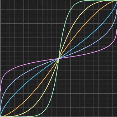
Remapping the unit interval into the unit interval by expanding the sides and compressing the center, and keeping 1/2 mapped to 1/2, that can be done with the gain() function. This was a common function in RSL tutorials (the Renderman Shading Language). k=1 is the identity curve, k<1 produces the classic gain() shape, and k>1 produces "s" shaped curces. The curves are symmetric (and inverse) for k=a and k=1/a.
float gain(float x, float k)
{
    const float a = 0.5*pow(2.0*((x<0.5)?x:1.0-x), k);
    return (x<0.5)?a:1.0-a;
}
# Parabola
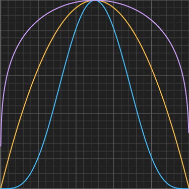
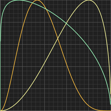
A nice choice to remap the 0..1 interval into 0..1, such that the corners are mapped to 0 and the center to 1. You can then rise the parabolar to a power k to control its shape.
float parabola( float x, float k )
{
    return pow( 4.0*x*(1.0-x), k );
}
# Power curve
This is a generalziation of the Parabola() above. It also maps the 0..1 interval into 0..1 by keeping the corners mapped to 0. But in this generalziation you can control the shape one either side of the curve, which comes handy when creating leaves, eyes, and many other interesting shapes.
float pcurve( float x, float a, float b )
{
    const float k = pow(a+b,a+b)/(pow(a,a)*pow(b,b));
    return k*pow(x,a)*pow(1.0-x,b);
}
Note that k is chosen such that pcurve() reaches exactly 1 at its maximum for illustration purposes, but in many applications the curve needs to be scaled anyways so the slow computation of k can be simply avoided.
# Sinc curve
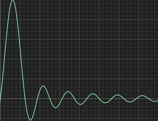
A phase shifted sinc curve (opens new window) can be useful if it starts at zero and ends at zero, for some bouncing behaviors (suggested by Hubert-Jan). Give k different integer values to tweak the amount of bounces. It peaks at 1.0, but that take negative values, which can make it unusable in some applications.
float sinc( float x, float k )
{
    const float a = PI*((k*x-1.0);
    return sin(a)/a;
}
# Falloff
A quadratic falloff, like those in physically based point lights, but reaching zero at a given distance "m" rather than just asymptotically reaching it at infinity. Great for range controlled shadows, etc.
float trunc_fallof( in float x, float m )
{
    x = 1.0/((x+1.0)*(x+1.0));
    m = 1.0/((m+1.0)*(m+1.0));
    return (x-m)/(1.0-m);
}